The central limit theorem states that, given a parent distribution of mean $\mu$ and variance $\sigma^2$, if you independently draw $k$ samples from this parent distribution, average them to get one value, then repeat this process over and over, the resulting distribution formed by these values will approach a normal distribution of mean $\mu$ and variance $\sigma^2/k$ as $k \to \infty$.

Because I have always had poor intuition for this theorem, below I’ll discuss (with very simple examples) how this convergence to normality occurs for different parent distributions, along with some illustrations.

Uniform distribution

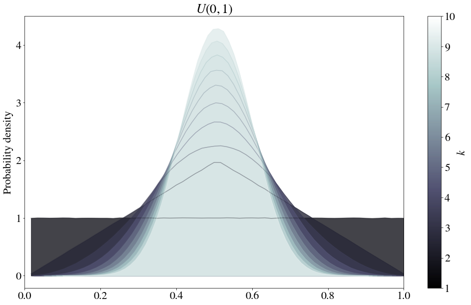
Consider a uniform distribution defined between 0 and 1 (note that an unbounded uniform distribution is a trivial example of a distribution with an infinite variance for which no convergence would occur).

The most curious feature is the kinked line that occurs when $k=2$. The functional form of this kinked line can be found theoretically. In particular, we need to obtain the total probability that two values $x_1$ and $x_2$ sum to a particular value $u$ (for now, this is defined between $0$ and $2$ – we will divide by $2$ later to turn this sum into an average). This can be written as follows:

$$P(u = x + y) = \int_{-\infty}^{\infty} P(x) P(u - x) \ dx$$

(note this is a convolution – for a fantastic, more thorough explanation of the above equation, see Understanding Convolutions by Christopher Olah). $P(x) = 1$, so the integrals should be quite simple. The only trick here is to solve for the piecewise behavior… $P(u - x)$ is only $1$ where $0 \leq u - x \leq 1$, or in other words, where $ -1 +u \leq x \leq u $, and $P(x)$ is only $1$ when $0 \leq x \leq 1$. Therefore, between $0 \leq u \leq 1$, we have

$$P(u) = \int_{0}^{u} dx = u$$

And for $u>1$, we have

$$P(u) = \int_{-1+u}^{1} dx = 2 - u$$

We can define $G(u)$, the probability density function for the average of two values $x_1$ and $x_2$, by moving the threshold to $u=1/2$ and doubling the density, as follows:

$$G(u) = \begin{cases} 4 u & 0 \leq u \leq 0.5 \\ 4 - 4u & 0.5 \leq u \leq 1 \\ 0 & \text{otherwise} \end{cases}$$

… consistent with our figure!

Beta distribution

The beta distribution is a normalized version of:

$$P(x) \sim x^{\alpha-1} (1-x)^{\beta -1}$$

Because it’s only defined between 0 and 1, it certainly satisfies the condition that the second moment is finite.

Log-normal distribution

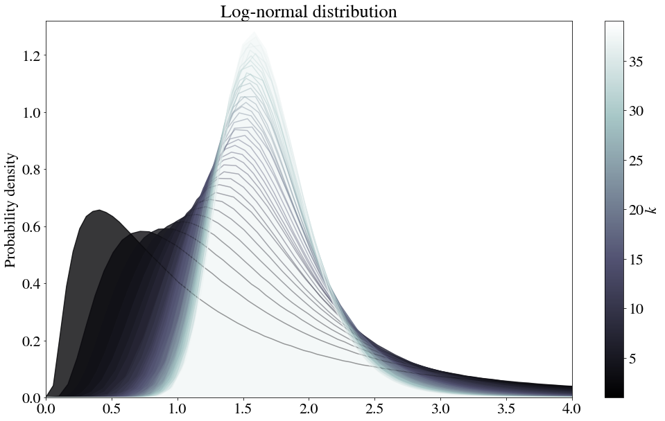
Curiously, this theorem also works for the log-normal distribution:

$$P(x) \sim \frac{1}{x} e^{- (\ln x - \mu)^2 / 2 \sigma^2}$$

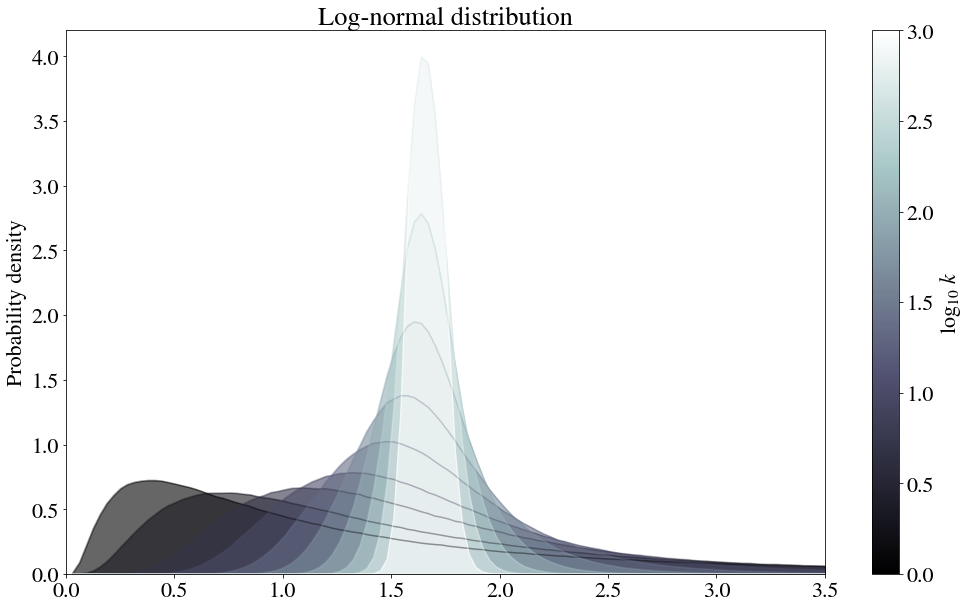
It takes a bit longer for the convergence to occur, so let’s try log-spacing the number of samples to average.

Because there are so many distributions that are log-normal, the central limit applied here has some strong practical ramifications. For example, if price distributions tend to be log-normal, then a revenue distribution for which multiple orders are placed could perhaps be more accurately described as one of these in-between shapes. Or, at a coarser scale, this could mean that the amount of money spent by a person each year is normally distributed.

Or, considering prices tend to be between power law or log normal, if log normality is observed, could it somehow be a step on the way to normalcy, from the summing of random independent variables that are power-law distributed? Let’s move onto power-law distributions to find out!

Pareto distributions

The “Pareto distribution” is a power law distribution $P(x) \sim 1/x^a$. To avoid the singularity at $x=0$, this is often shifted over, or only defined starting at $x=1$ (or a different value, depending on the scaling).

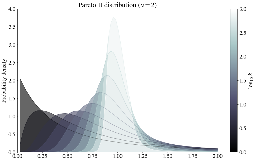
numpy.random.pareto is used here. The formula appears to be:

$$P(x) \sim \frac{1}{(1+x)^{\alpha+1}}$$

For $\alpha = 2$, for which the variance is finite, the normal distribution appears.

The first few steps indeed look somewhat log-normal!

However, for $\alpha =1$, for which the variance is infinite, no normal distribution appears to be in sight.

While this empirical test does seem to indicate that no convergence to a normal distribution occurs, it does still converge to an alpha-stable distribution.

Final notes

Note that the density of the sum of two independent real-valued random variables equals the convolution of the density functions of the original variables. We could therefore recreate these graphs analytically.

A couple remaining open questions:

• How does the peak of the pdf change with $N$?
  This peak increases in height as the distribution narrows as mentioned above, but for the log-normal case it decreases before it increases.
• Why does the power law appear to converge slower than the other distributions?
  Explicitly, the question amounts to: how does changing the functional form of a convolving function affect the convergence of a series of such convolutions to the convergent distribution? A simple way to approach this would be to check the Kolmogorov-Smirnov distance between the the converging distribution and the normal distribution (note: the Berry-Esseen theorem appears to do just that!), but perhaps there exists a more elegant way to do this, while also answering the first question above…